统计推断框架
infer 包统一推断
统计建模篇Statistical Inference: A Tidy Approach
案例1:你会给爱情片还是动作片高分?

这是一个关于电影评分的数据集[^2],
[^2]: <https://github.com/hadley/ggplot2movies/blob/master/R/movies.R>
R
library(tidyverse)
d <- ggplot2movies::movies
d
数据集包含58788 行 和 24 变量
| variable | description |
|---|---|
| title | 电影名 |
| year | 发行年份 |
| budget | 预算金额 |
| length | 电影时长 |
| rating | 平均得分 |
| votes | 投票人数 |
| r1-10 | 各分段投票人占比 |
| mpaa | MPAA 分级 |
| action | 动作片 |
| animation | 动画片 |
| comedy | 喜剧片 |
| drama | 戏剧 |
| documentary | 纪录片 |
| romance | 爱情片 |
| short | 短片 |
我们想看下爱情片与动作片(不是爱情动作片)的平均得分是否显著不同。
- 首先我们简单的整理下数据,主要是剔除既是爱情片又是动作片的电影
R
movies_genre_sample <- d %>%
select(title, year, rating, Action, Romance) %>%
filter(!(Action == 1 & Romance == 1)) %>%
mutate(genre = case_when(
Action == 1 ~ "Action",
Romance == 1 ~ "Romance",
TRUE ~ "Neither"
)) %>%
filter(genre != "Neither") %>%
select(-Action, -Romance) %>%
group_by(genre) %>%
#slice_sample(n = 34) %>% # sample size = 34
slice_head(n = 34) %>%
ungroup()
movies_genre_sample- 先看下图形
R
movies_genre_sample %>%
  ggplot(aes(x = genre, y = rating)) +
  geom_boxplot() +
geom_jitter()- 看下两种题材电影评分的分布
R
movies_genre_sample %>%
  ggplot(mapping = aes(x = rating)) +
  geom_histogram(binwidth = 1, color = "white") +
facet_grid(vars(genre))- 统计两种题材电影评分的均值
R
summary_ratings <- movies_genre_sample %>%
  group_by(genre) %>%
  summarize(
    mean = mean(rating),
    std_dev = sd(rating),
    n = n()
  )
summary_ratings
传统的基于频率方法的t检验
假设:
- 零假设:
- $H_0: \mu_{1} - \mu_{2} = 0$
- 备选假设:
- $H_A: \mu_{1} - \mu_{2} \neq 0$
两种可能的结论:
- 拒绝 $H_0$
- 不能拒绝 $H_0$
R
t_test_eq <- t.test(rating ~ genre,
  data = movies_genre_sample,
  var.equal = TRUE
) %>%
  broom::tidy()
t_test_eq
R
t_test_uneq <- t.test(rating ~ genre,
  data = movies_genre_sample,
  var.equal = FALSE
) %>%
  broom::tidy()
t_test_uneq
infer:基于模拟的检验
所有的假设检验都符合这个框架[^2]:
[^2]: <http://allendowney.blogspot.com/2016/06/there-is-still-only-one-test.html>
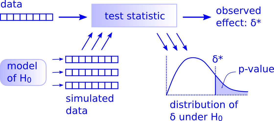
- 实际观察的差别
R
library(infer)

obs_diff <- movies_genre_sample %>%
  specify(formula = rating ~ genre) %>%
  calculate(
    stat = "diff in means",
    order = c("Romance", "Action")
  )
obs_diff- 模拟
R
null_dist <- movies_genre_sample %>%
  specify(formula = rating ~ genre) %>%
  hypothesize(null = "independence") %>%
  generate(reps = 5000, type = "permute") %>%
  calculate(
    stat = "diff in means",
    order = c("Romance", "Action")
  )
head(null_dist)- 可视化
R
null_dist %>%
  visualize()
R
null_dist %>%
  visualize() +
  shade_p_value(obs_stat = obs_diff, direction = "both")
# shade_p_value(bins = 100, obs_stat = obs_diff, direction = "both")- 计算p值
R
pvalue <- null_dist %>%
  get_pvalue(obs_stat = obs_diff, direction = "two_sided")

pvalue- 结论
在构建的虚拟($\Delta = 0$)的平行世界里,出现实际观察值([R表达式])的概率为([R表达式])。 如果以(p \< 0.05)为标准,我们看到p_value < 0.05, 那我们有足够的证据证明,H0不成立,即爱情电影和动作电影的评分均值存在显著差异,具体来说,动作电影的平均评分要比爱情电影低些。
案例2: 航天事业的预算有党派门户之见?
美国国家航空航天局的预算是否存在党派门户之见?
R
gss <- read_rds("./demo_data/gss.rds")

gss %>%
  select(NASA, party) %>%
  count(NASA, party) %>%
  head(8)
R
gss %>%
  ggplot(aes(x = party, fill = NASA)) +
  geom_bar()
假设:
- 零假设 $H_0$:
- 不同党派对预算的态度的构成比(TOO LITTLE, ABOUT RIGHT, TOO MUCH) 没有区别
- 备选假设 $H_a$:
- 不同党派对预算的态度的构成比(TOO LITTLE, ABOUT RIGHT, TOO MUCH) 存在区别
两种可能的结论:
- 拒绝 $H_0$
- 不能拒绝 $H_0$
传统的方法
R
chisq.test(gss$party, gss$NASA)或者
R
gss %>%
  chisq_test(NASA ~ party) %>%
  dplyr::select(p_value) %>%
  dplyr::pull()
infer:Simulation-based tests
R
obs_stat <- gss %>%
  specify(NASA ~ party) %>%
  calculate(stat = "Chisq")
obs_stat
R
null_dist <- gss %>%
  specify(NASA ~ party) %>%                     # (1)
  hypothesize(null = "independence") %>%        # (2)
    generate(reps = 5000, type = "permute") %>% # (3)
  calculate(stat = "Chisq")                     # (4)
null_dist
R
null_dist %>%
  visualize() +
  shade_p_value(obs_stat = obs_stat, method = "both", direction = "right")
R
null_dist %>%
  get_pvalue(obs_stat = obs_stat, direction = "greater")
看到 p_value > 0.05,不能拒绝 $H_0$,我们没有足够的证据证明党派之间有显著差异
using ggstatsplot::ggbarstats()
R
library(ggstatsplot)

gss %>%
  ggbarstats(
    x = party,
    y = NASA
)
案例3:原住民中的女学生多?
案例 quine 数据集有 146 行 5 列,包含学生的生源、文化、性别和学习成效,具体说明如下
- Eth: 民族背景:原住民与否 (是"A"; 否 "N")
- Sex: 性别
- Age: 年龄组 ("F0", "F1," "F2" or "F3")
- Lrn: 学习者状态(平均水平 "AL", 学习缓慢 "SL")
- Days:一年中缺勤天数
R
td <- MASS::quine %>%
  as_tibble() %>%
  mutate(
    across(c(Sex, Eth), as_factor)
  )
td
从民族背景有两组(A, N)来看,性别为 F 的占比 是否有区别?
R
td %>% count(Eth, Sex)传统方法
R
prop.test(table(td$Eth, td$Sex), correct = FALSE)基于模拟的方法
被解释变量 sex 中F的占比,解释变量中两组(A,N)
R
obs_diff <- td %>%
  specify(Sex ~ Eth, success = "F") %>%
  calculate(
    stat = "diff in props",
    order = c("A", "N")
  )

obs_diff
R
null_distribution <- td %>%
  specify(Sex ~ Eth, success = "F") %>%
  hypothesize(null = "independence") %>%
  generate(reps = 5000, type = "permute") %>%
  calculate(stat = "diff in props", order = c("A", "N"))
R
null_distribution %>%
  visualize()
R
pvalue <- null_distribution %>%
  get_pvalue(obs_stat = obs_diff, direction = "both")

pvalue
R
null_distribution %>%
get_ci(level = 0.95, type = "percentile")宏包infer
我比较喜欢infer宏包的设计思想,它把统计推断分成了四个步骤
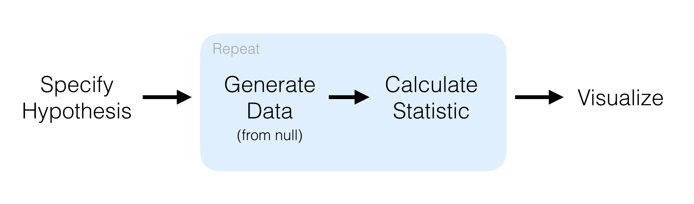
下图可以更好的帮助我们理解infer的工作流程 !图片
specify()指定解释变量和被解释变量 (y ~ x)hypothesize()指定零假设 (比如,independence=y和x彼此独立)generate()从基于零假设的平行世界中抽样:- 指定每次重抽样的类型,通俗点讲就是数据洗牌,重抽样
type = "bootstrap"(有放回的),对应的零假设往往是null = "point" ; 重抽样type = "permuting"(无放回的),对应的零假设往往是null = "independence", 指的是y和x之间彼此独立的,因此抽样后会重新排列,也就说原先 value1-group1 可能变成了value1-group2,(因为我们假定他们是独立的啊,这种操作,也不会影响y和x的关系) - 指定多少组 (
reps = 1000) calculate()计算每组(reps)的统计值 (stat = "diff in props")visualize()可视化,对比零假设的分布与实际观察值.
下面是我自己对重抽样的理解 !图片
更多
更多统计推断的内容可参考
- <http://infer.netlify.com>
- <https://moderndive.netlify.com/index.html>
- <https://moderndive.com/index.html>
- <https://github.com/tidymodels/infer>
R
# remove the objects
# rm(list=ls())
rm(d, gss, movies_genre_sample, null_dist, null_distribution, obs_diff, obs_stat, pvalue, summary_ratings, t_test_eq, t_test_uneq, td)
R
pacman::p_unload(pacman::p_loaded(), character.only = TRUE)