企鹅数据集

经典数据集全面分析

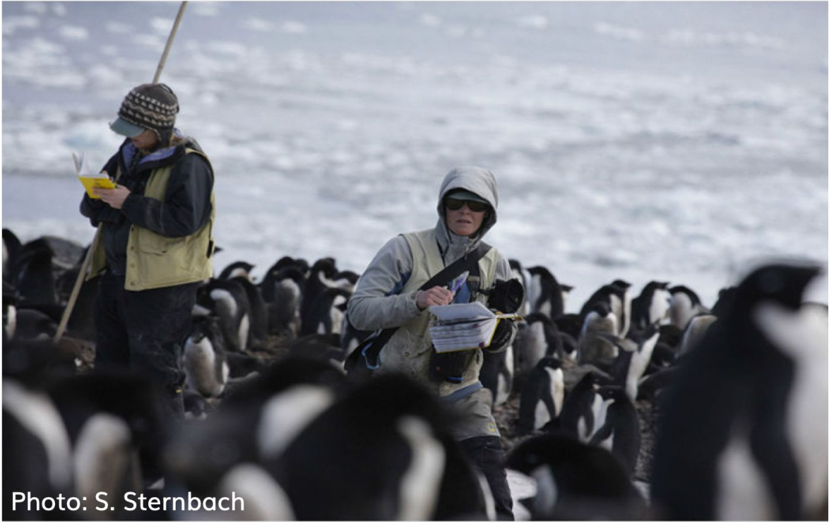
应用篇

今天讲一个关于企鹅的数据故事。这个故事来源于科考人员记录的大量企鹅体征数据，图片来源这里.

数据

导入数据

可通过宏包palmerpenguins::penguins获取数据，也可以读取本地penguins.csv文件，我们采取后面一种方法：

library(tidyverse)
penguins <- read_csv("./demo_data/penguins.csv") %>%
  janitor::clean_names()

penguins %>%
  head()

变量含义

variable	class	description
species	integer	企鹅种类 (Adelie, Gentoo, Chinstrap)
island	integer	所在岛屿 (Biscoe, Dream, Torgersen)
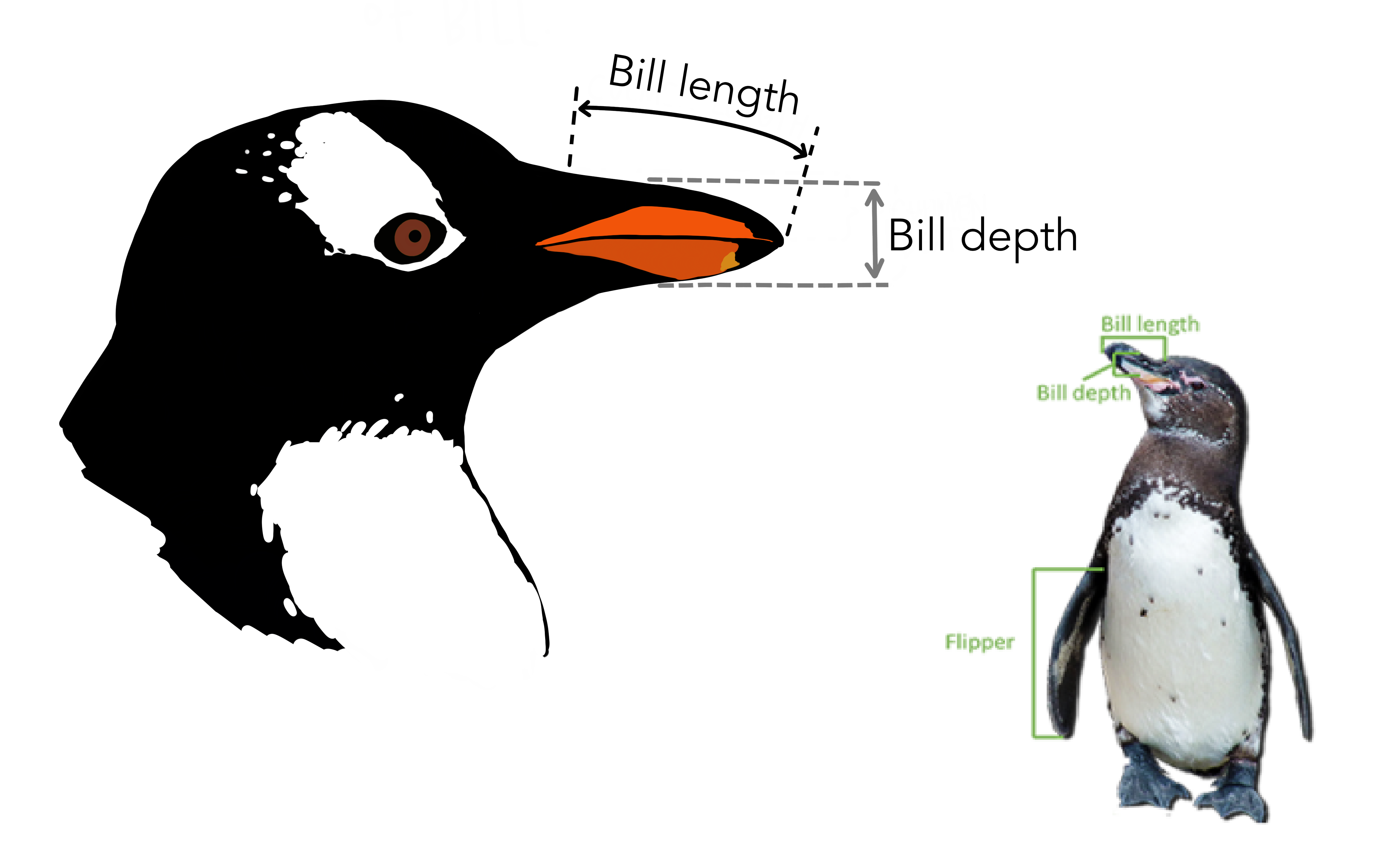
bill_length_mm	double	嘴峰长度 (单位毫米)
bill_depth_mm	double	嘴峰深度 (单位毫米)
flipper_length_mm	integer	鰭肢长度 (单位毫米)
body_mass_g	integer	体重 (单位克)
sex	integer	性别
year	integer	记录年份

数据清洗

检查缺失值(NA)这个很重要！

penguins %>% summarise(
  across(everything(), ~ sum(is.na(.)))
)

有缺失值的地方找出来看看

penguins %>% filter_all(
  any_vars(is.na(.))
)

发现共有11行至少有一处有缺失值，于是我们就删除这些行

penguins <- penguins %>% drop_na()
penguins

探索性分析

大家可以提出自己想探索的内容：

每种类型企鹅有多少只？
每种类型企鹅各种属性的均值和分布？
嘴峰长度和深度的关联？
体重与翅膀长度的关联？
嘴峰长度与嘴峰深度的比例？
不同种类的宝宝，体重具有显著性差异？
这体征中哪个因素对性别影响最大？
...

每种类型企鹅有多少只

penguins %>%
  count(species, sort = T)

每个岛屿有多少企鹅？

penguins %>%
  count(island, sort = T)

每种类型企鹅各种体征属性的均值和分布

penguins %>%
  group_by(species) %>%
  summarize(across(where(is.numeric), mean, na.rm = TRUE))

每种类型企鹅的嘴峰长度的分布

penguins %>%
  ggplot(aes(x = bill_length_mm)) +
  geom_density() +
  facet_wrap(vars(species), scales = "free")

每种类型企鹅的嘴峰长度的分布（分性别）

penguins %>%
  ggplot(aes(x = bill_length_mm)) +
  geom_density(aes(fill = sex)) +
  facet_wrap(vars(species), scales = "free")

男宝宝的嘴巴要长些，哈哈。

来张更好看点的

penguins %>%
  ggplot(aes(x = bill_length_mm, fill = sex)) +
  geom_histogram(
    position = "identity",
    alpha = 0.7,
    bins = 25
  ) +
  scale_fill_manual(values = c("#66b3ff", "#8c8c8c")) +
  ylab("number of penguins") +
  xlab("length (mm)") +
  theme_minimal() +
  theme(
    legend.position = "bottom",
    legend.text = element_text(size = 11),
    legend.title = element_blank(),
    panel.grid.minor = element_blank(),
    axis.title = element_text(color = "white", size = 10),
    plot.title = element_text(size = 20),
    plot.subtitle = element_text(size = 12, hjust = 1)
  ) +
  facet_wrap(vars(species), scales = "free")

同理，可以画出其他属性的分布。当然，我更喜欢用山峦图来呈现不同分组的分布，因为竖直方向可以更方便比较

library(ggridges)
penguins %>%
  ggplot(aes(x = bill_length_mm, y = species, fill = species)) +
  ggridges::geom_density_ridges()

同样，我们也用颜色区分下性别，这样不同种类、不同性别企鹅的嘴峰长度分布一目了然

penguins %>%
  ggplot(aes(x = bill_length_mm, y = species, fill = sex)) +
  geom_density_ridges(alpha = 0.5)

同样的代码，类似地画个其他体征的分布，

penguins %>%
  ggplot(aes(x = bill_depth_mm, fill = species)) +
  ggridges::geom_density_ridges(aes(y = species))

penguins %>%
  ggplot(aes(x = bill_depth_mm, fill = sex)) +
  ggridges::geom_density_ridges(aes(y = species))

penguins %>%
  ggplot(aes(x = body_mass_g, y = species, fill = sex)) +
  ggridges::geom_density_ridges(alpha = 0.5)

但这样一个特征一个特征的画，好麻烦。你知道程序员都是偷懒的，于是我们还有更骚的操作

penguins %>%
  dplyr::select(species, bill_length_mm:body_mass_g) %>%
  pivot_longer(-species, names_to = "measurement", values_to = "value") %>%
  ggplot(aes(x = value)) +
  geom_density(aes(color = species, fill = species), size = 1.2, alpha = 0.2) +
  facet_wrap(vars(measurement), ncol = 2, scales = "free")

penguins %>%
  dplyr::select(species, bill_length_mm:body_mass_g) %>%
  pivot_longer(-species, names_to = "measurement", values_to = "value") %>%
  ggplot(aes(x = species, y = value)) +
  geom_boxplot(aes(color = species, fill = species), size = 1.2, alpha = 0.2) +
  facet_wrap(vars(measurement), ncol = 2, scales = "free")

penguins %>%
  dplyr::select(species, bill_length_mm:body_mass_g) %>%
  pivot_longer(-species, names_to = "measurement", values_to = "value") %>%
  ggplot(aes(x = value, y = species, fill = species)) +
  ggridges::geom_density_ridges() +
  facet_wrap(vars(measurement), scales = "free")

penguins %>%
  dplyr::select(species,sex, bill_length_mm:body_mass_g) %>%
  pivot_longer(
    -c(species, sex), 
    names_to = "measurement", 
    values_to = "value"
    ) %>%
  ggplot(aes(x = value, y = species, fill = sex)) +
  ggridges::geom_density_ridges() +
  facet_wrap(vars(measurement), scales = "free")

我若有所思的看着这张图，似乎看到了一些特征（pattern）了。

嘴峰长度和深度的关联

嘴巴越长，嘴巴也会越厚？

penguins %>%
  ggplot(aes(
    x = bill_length_mm, y = bill_depth_mm,
    shape = species, color = species
  )) +
  geom_point()

我们把不同的种类，用不同的颜色区分看看

penguins %>%
  ggplot(aes(
    x = bill_length_mm, y = bill_depth_mm,
    shape = species, color = species
  )) +
  geom_point(aes(size = body_mass_g))

感觉这是一个辛普森佯谬，我们画图看看

penguins %>%
  ggplot(aes(x = bill_length_mm, y = bill_depth_mm)) +
  geom_point(aes(color = species, shape = species)) +
  geom_smooth(method = lm) +
  geom_smooth(method = lm, aes(color = species))

体重与翅膀长度的关联

翅膀越长，体重越大？

penguins %>%
  group_by(species, island, sex) %>%
  ggplot(aes(
    x = body_mass_g, y = reorder(species, -body_mass_g),
    color = species
  )) +
  geom_jitter(position = position_jitter(seed = 2020, width = 0.2), alpha = 0.4, size = 2) +
  stat_summary(fun = mean, geom = "point", size = 5, alpha = 1)

library(ggtext)
penguins %>%
  ggplot(aes(flipper_length_mm, body_mass_g, group = species)) +
  geom_point(aes(colour = species, shape = species), alpha = 0.7) +
  scale_color_manual(values = c("darkorange", "purple", "cyan4")) +
  labs(
    title = "Penguin Size, Palmer Station LTER",
    subtitle = "Flipper length and body mass for <span style = 'color:darkorange;'>Adelie</span>, <span style = 'color:purple;'>Chinstrap</span> and <span style = 'color:cyan4;'>Gentoo</span> Penguins",
    x = "flipper length (mm)",
    y = "body mass (g)"
  ) +
  theme_minimal() +
  theme(
    legend.position = "none",
    # text = element_text(family = "Futura"),
    # (I only have 'Light' )
    plot.title = element_text(size = 16),
    plot.subtitle = element_markdown(), # element_markdown from `ggtext` to parse the css in the subtitle
    plot.title.position = "plot",
    plot.caption = element_text(size = 8, colour = "grey50"),
    plot.caption.position = "plot"
  )

不同种类的宝宝，体重具有显著性差异？

先分组计算体重的均值和标准差

penguins %>%
  group_by(species) %>%
  summarise(
    count = n(),
    mean_body_mass = mean(body_mass_g),
    sd_body_mass = sd(body_mass_g)
  )

penguins %>%
  ggplot(aes(x = species, y = body_mass_g)) +
  geom_boxplot() +
  geom_jitter()

用统计方法验证下我们的猜测吧。记住，我们是有科学精神的的人！

参数检验

one-way ANOVA(要求等方差)

stats::aov(formula = body_mass_g ~ species, data = penguins) %>%
  summary()

p-value 很小，说明不同种类企鹅之间体重是有显著差异的，但aov只给出了species在整体上引起了体重差异（只要有任意两组之间有显著差异，aov给出的p-value都很小），如果想知道不同种类两两之间是否有显著差异，这就需要用到TukeyHSD().

one-way ANOVA(不要求等方差)，相关介绍看here

oneway.test(body_mass_g ~ species, data = penguins)

stats::aov(formula = body_mass_g ~ species, data = penguins) %>%
  TukeyHSD(which = "species") %>%
  broom::tidy()

表格第一行instrap-Adelie 的 p-value = 0.916，没通过显著性检验；而Gentoo-Adelie 和 Gentoo-Chinstrap 他们的p-value都接近0，通过显著性检验，这和图中的结果是一致的。

作为统计出生的R语言，有很多宏包可以帮助我们验证我们的结论，我这里推荐可视化学统计的宏包ggstatsplot宏包将统计分析的结果写在图片里，统计结果和图形融合在一起，让统计结果更容易懂了。（使用这个宏包辅助我们学习统计）

library(ggstatsplot)

penguins %>%
  ggstatsplot::ggbetweenstats(
    x = species, # > 2 groups
    y = body_mass_g,
    type = "parametric",
    pairwise.comparisons = TRUE, 
    pairwise.display = "all",
    messages = FALSE,
    var.equal = FALSE
  )

非参数检验

嘴峰长度与嘴峰深度的比例

penguins %>%
  mutate(ratio = bill_length_mm / bill_depth_mm) %>%
  group_by(species) %>%
  summarise(mean = mean(ratio))

penguins %>%
  mutate(ratio = bill_length_mm / bill_depth_mm) %>%
  ggplot(aes(x = ratio, fill = species)) +
  ggridges::geom_density_ridges(aes(y = species))

男宝宝和女宝宝颜色区分下，代码只需要修改一个地方，留给大家自己实践下吧。

建立模型

建模需要标准化数据，并对分类变量（比如sex）编码为 1 和 0; （这是第二个好习惯）

scale_fun <- function(x) {  
  (x - mean(x)) / sd(x)
}

d <- penguins %>%
  select(sex, species, bill_length_mm:body_mass_g) %>%
  mutate(
    across(where(is.numeric), scale_fun)
  ) %>%
  mutate(male = if_else(sex == "male", 1, 0))
d

按照species分组后，对flipper_length_mm标准化？这样数据会聚拢到一起了喔, 还是不要了

penguins %>%
  select(sex, species, bill_length_mm:body_mass_g) %>%
  group_by(species) %>%
  mutate(
    across(where(is.numeric), scale_fun)
  ) %>%
  ungroup()

model_01

我们将性别sex视为响应变量，其他变量为预测变量。这里性别变量是二元的（0 或者 1），所以我们用logistic回归

logit_mod1 <- glm(
  male ~ 1 + species + bill_length_mm + bill_depth_mm +
    flipper_length_mm + body_mass_g,
  data = d,
  family = binomial(link = "logit")
)

summary(logit_mod1)

计算每个变量的平均边际效应

library(margins)

logit_mod1_m <- logit_mod1 %>% 
 margins() %>% 
 summary() %>% 
 as_tibble()

logit_mod1_m

logit_mod1_m %>%
  ggplot(aes(
    x = reorder(factor, AME),
    y = AME, ymin = lower, ymax = upper
  )) +
  geom_hline(yintercept = 0, color = "gray80") +
  geom_pointrange() +
  coord_flip() +
  labs(x = NULL, y = "Average Marginal Effect")

library(ggeffects)
ggpredict(logit_mod1, terms = "bill_length_mm")

model_02

library(brms)

brms_mod2 <- brm(
  male ~ 1 + bill_length_mm + bill_depth_mm + flipper_length_mm + body_mass_g + (1 | species),
  data = d,
  family = binomial(link = "logit")
)

summary(brms_mod2)

library(ggeffects)
ggpredict(brms_mod2, "bill_depth_mm [all]") %>%
  plot()

model_03

penguins %>%
  ggplot(aes(x = flipper_length_mm, y = bill_length_mm, color = species)) +
  geom_point()

brms_mod3 <- brm(bill_length_mm ~ flipper_length_mm + (1|species),
  data = penguins
)

penguins %>%
  group_by(species) %>%
  modelr::data_grid(flipper_length_mm) %>%
  tidybayes::add_fitted_draws(brms_mod3, n = 100) %>%
  ggplot() +
  geom_point(
    data = penguins,
    aes(flipper_length_mm, bill_length_mm, color = species, shape = species)
  ) +
  geom_line(aes(flipper_length_mm, .value, group = interaction(.draw, species), color = species), alpha = 0.1)

# remove the objects
# rm(list=ls())
rm(d, logit_mod1, logit_mod1_m, penguins, scale_fun)

pacman::p_unload(pacman::p_loaded(), character.only = TRUE)