房价预测 — 数据科学中的 R 语言

数据故事

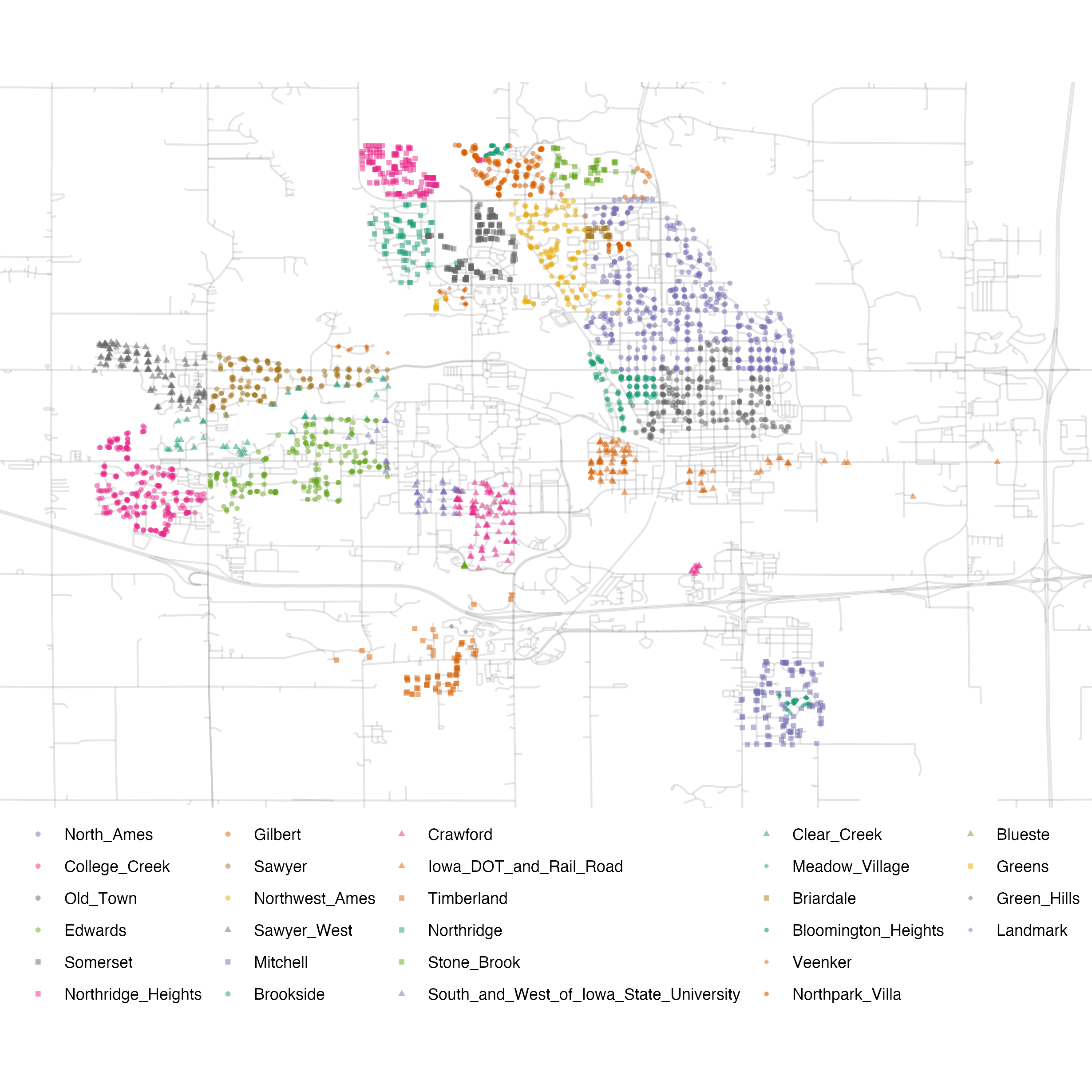
这是一份Ames房屋数据，您可以把它想象为房屋中介推出的成都市武侯区、锦江区以及高新区等各区县的房屋信息

R

library(tidyverse)
ames <- read_csv("./demo_data/ames_houseprice.csv") %>% 
        janitor::clean_names()

glimpse(ames)

感谢曾倬同学提供的解释说明文档

R

explanation <- readxl::read_excel("./demo_data/ames_houseprice_explanation.xlsx")
explanation %>% 
  knitr::kable()

探索设想

读懂数据描述，比如
房屋设施 (bedrooms, garage, fireplace, pool, porch, etc.),
地理位置 (neighborhood),
土地信息 (zoning, shape, size, etc.),
品相等级
出售价格

探索影响房屋价格的因素
必要的预处理（缺失值处理、标准化、对数化等等）
必要的可视化（比如价格分布图等）
必要的统计（比如各地区房屋价格的均值）
合理选取若干预测变量，建立多元线性模型，并对模型结果给出解释
房屋价格与预测变量（房屋大小、在城市的位置、房屋类型、与街道的距离）

变量选取

我们选取下列变量：

lot_frontage, 建筑离街道的距离
lot_area, 占地面积
neighborhood, 建筑在城市的位置
gr_liv_area, 地上居住面积
bldg_type, 住宅类别(联排别墅、独栋别墅...)
year_built 房屋修建日期

R

d <- ames %>% 
  select(sale_price, 
         lot_frontage,   
         lot_area,      
         neighborhood,   
         gr_liv_area,   
         bldg_type,      
         year_built      
         )
d

缺失值处理

R

d %>% 
  summarise(
    across(everything(), function(x) sum(is.na(x)) )
  )

找出来看看

R

d %>% 
  filter_all(
    any_vars(is.na(.))
  )

R

library(visdat)

d %>% vis_dat()

如果不选择lot_frontage 就不会有缺失值，如何选择，自己抉择

R

d %>% 
  select(-lot_frontage) %>% 
  visdat::vis_dat()

我个人觉得这个变量很重要，所以还是保留，牺牲一点样本量吧

R

d <- d %>% 
  drop_na()

R

d %>% visdat::vis_dat()

预处理

标准化

R

standard <- function(x) {
  (x - mean(x)) / sd(x)
}

d %>% 
  mutate(
    across(where(is.numeric), standard),
    across(where(is.character), as.factor)
  )

对数化

R

d %>% 
  mutate(
    log_sale_price = log(sale_price)
  )

R

d %>% 
  mutate(
    across(where(is.numeric), log),
    across(where(is.character), as.factor)
  )

标准化 vs 对数化

选择哪一种，我们看图说话

R

d %>% 
  ggplot(aes(x = sale_price)) +
  geom_density()

R

d %>% 
  ggplot(aes(x = log(sale_price))) +
  geom_density()

我们选择对数化，并保存结果

R

d <- d %>% 
  mutate(
    across(where(is.numeric), 
           .fns = list(log = log), 
           .names = "{.fn}_{.col}"
           ),
    across(where(is.character), as.factor)
  )

有趣的探索

各区域的房屋价格均值

R

d %>% count(neighborhood)

R

d %>% 
  group_by(neighborhood) %>% 
  summarise(
    mean_sale = mean(sale_price)
  ) %>% 
  
  ggplot(
    aes(x = mean_sale, y = fct_reorder(neighborhood, mean_sale))
  ) +
  geom_col(aes(fill = mean_sale &lt; 150000), show.legend = FALSE) +
  geom_text(aes(label = round(mean_sale, 0)), hjust = 1) +
  # scale_x_continuous(
  #   expand = c(0, 0),
  #   breaks = c(0, 100000, 200000, 300000),
  #   labels = c(0, "1w", "2w", "3w")    
  #   ) +
  scale_x_continuous(
    expand = c(0, 0),
    labels = scales::dollar
  ) +
  scale_fill_viridis_d(option = "D") + 
  theme_classic() +
  labs(x = NULL, y = NULL)

房屋价格与占地面积

R

d %>%
  ggplot(aes(x = log_lot_area, y = log_sale_price)) +
  geom_point(colour = "blue") +
  geom_smooth(method = lm, se = FALSE, formula = "y ~ x")

R

d %>%
  ggplot(aes(x = log_lot_area, y = log_sale_price)) +
  geom_point(aes(colour = neighborhood)) +
  geom_smooth(method = lm, se = FALSE, formula = "y ~ x")

R

d %>%
  ggplot(aes(x = log_lot_area, y = log_sale_price)) +
  geom_point(colour = "blue") +
  geom_smooth(method = lm, se = FALSE, formula = "y ~ x", fullrange = TRUE) +
  facet_wrap(~neighborhood) +
  theme(strip.background = element_blank())

房屋价格与房屋居住面积

R

d %>%
  ggplot(aes(x = log_gr_liv_area, y = log_sale_price)) +
  geom_point(aes(colour = neighborhood)) +
  geom_smooth(method = lm, se = FALSE, formula = "y ~ x")

R

d %>%
  ggplot(aes(x = log_gr_liv_area, y = log_sale_price)) +
  geom_point() +
  geom_smooth(method = lm, se = FALSE, formula = "y ~ x", fullrange = TRUE) +
  facet_wrap(~neighborhood) +
  theme(strip.background = element_blank())

车库与房屋价格

车库大小是否对销售价格有帮助?

R

ames %>% 
  #select(garage_cars, garage_area, sale_price) %>% 
  ggplot(aes(x = garage_area, y = sale_price)) +
  geom_point(
    data = select(ames, -garage_cars),
    color = "gray50"
  ) +
  geom_point(aes(color = as_factor(garage_cars))) +
  facet_wrap(vars(garage_cars)) +
  theme(legend.position = "none") +
  ggtitle("This is the influence of garage for sale price")

建模

R

lm(log_sale_price ~ 1 + log_gr_liv_area + neighborhood, data = d) %>% 
  broom::tidy()

R

library(lme4)
lmer(log_sale_price ~ 1 + log_gr_liv_area + (log_gr_liv_area | neighborhood), 
    data = d) %>% 
   broom.mixed::tidy()

R

# remove the objects
# ls() %>% stringr::str_flatten(collapse = ", ")
rm(ames, d, explanation)

R

pacman::p_unload(pacman::p_loaded(), character.only = TRUE)